8. Output
8.1. Concepts
SPIERSview: SPIERSedit does not directly visualise models in three dimensions, but instead exports models in compact ‘.spv’ file format, for viewing in SPIERSview (see SPIERSview manual). SPIERSview also provides facilities to export models as geometries to other software.
Output Objects: SPIERSedit exports a series of Output Objects, which are listed in the Objects tab of the Output panel; these are defined by the user as combinations of masks and (for multi-segment datasets) segments. The object will consist of all pixels assigned to any of these segments that fall into any of these masks. For instance, an object might list two masks and a ‘void’ segment; it would then comprise any void pixels with either of the two masks. In most cases however output objects consist of a single mask and segment, and represent all pixels in that segment and that mask. By default a single object is created, representing all pixels in the default mask and the default segment.
Output Downsampling: In addition to the dataset downsampling described in the Basic Concepts section, SPIERSedit supports a second form of downsampling performed at output time. This output downsampling applies only to the model exported to SPIERSview, and provides performance gains in SPIERSview as it reduced the complexity of the model to be displayed. Like dataset downsampling, output downsampling is defined as an XY and a Z setting. While XY downsampling works in the same way for both dataset and output downsampling, Z downsampling does not. A Z-downsampled dataset simply skips files – for example if Z downsampling is set to 3, only every third file in the sequence is used. Z-downsampling at output instead merges files; if set to 3, each set of 3 files is merged at output to determine whether any individual pixel is ‘on’ or ‘off’. Output downsampling is additive to dataset downsampling – if the dataset is downsampled by a factor of 2 and the output is also a downsampled by a factor of 2, it will in fact be downsampled by a factor of four from the source data.
Output Cache: Outputting models can be time consuming, as SPIERSedit needs to process data for all slices in the dataset. However once an output has been performed, SPIERSedit stores (caches) output information for each slice; for subsequent output operations only slices that have been altered are processed, and hence output is normally far quicker. Certain operations (e.g. creating or deleting a new output object) reset this cache.
8.2. Settings Tab
The Settings Tab of the Output panel (see Fig. 15, left) was introduced under Basic Concepts.
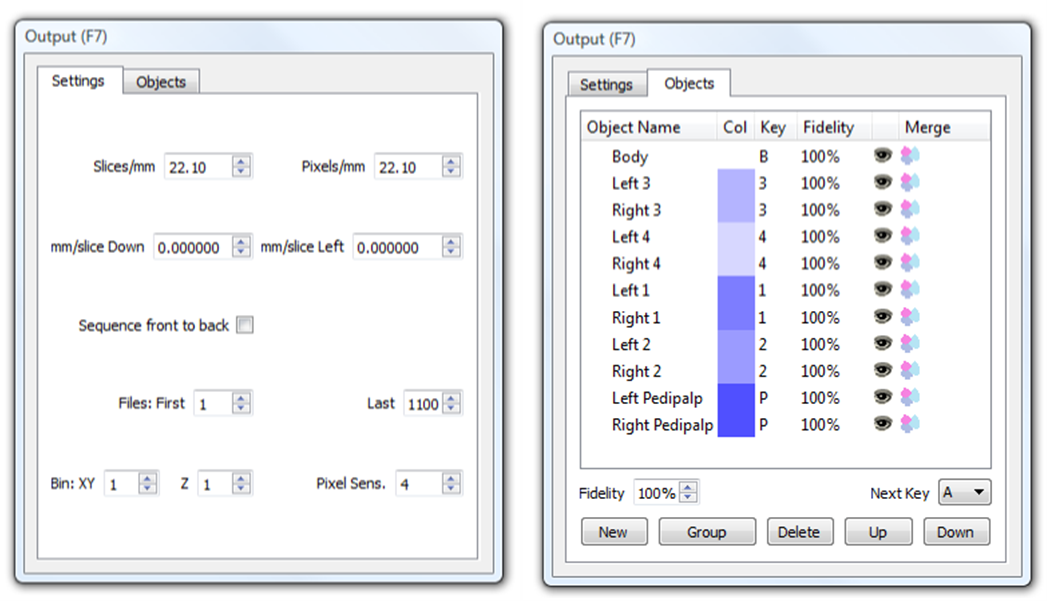
Figure 15. The Output Panel.* Left; Settings Tab. Right; Object Tab.
Slices/mm, Pixels/mm, Sequence front to back: See Basic Concepts (above).
mm/slice Down and mm/slice Left: See Deskewing (below).
Files: First and Last: restricts output to part of the dataset in terms of position in the Z direction; by default all files are included, but often a restricted portion only need be rendered at any one time, and including fewer files will normally speed up the output and rendering process.
Bin: XY and Z: These are the settings for output downsampling within each image (XY) and between images (Z).
Pixel Sens.: This is pixel sensitivity; it controls how output downsampling combines pixels. With output downsampling on (XY or Z values > 1), each voxel (3D pixel) output is assembled from Z x XY x XY threshold image pixels, each of which may be either ‘on’ or ‘off’. Pixel sensitivity is the number of threshold image pixels that need to be on before the voxel is turned on. For example if XY and Z are each 3, a cube of 3 x 3 x 3 = 27 pixels will be reduced to a single voxel. If Pixel Sens. is set to 1, only one of these 27 pixels need be on to turn the voxel on. If Pixel Sens. Is set to 14, over half would need to be turned on. If in doubt, leave Pixel Sens. at 1; using higher values can however help to reduce noise caused by sporadic scattered pixels.
8.3. Objects Tab
The Objects tab of the Output panel (see Fig. 15, Right) provides a list of output objects that that works in a manner similar to the Masks panel.
Object Name: This column provides a reference name for the object, which will appear in the Objects Panel of SPIERSview. Edit by double-clicking. Hovering the mouse over the name of an output object gives a list of the Masks and Segments that comprise it.
Col: The item colour in SPIERSview; edit by double-clicking. Note that groups can have a colour, though this is only used if they are merged (see below).
Key: The keyboard shortcut key that will be used to show/hide the object in SPIERSview ([-] means no key assigned). The Next Key dropdown below the main list is the key that will be assigned to the next object created.
Fidelity: The SPIERSview model fidelity; values of less than 100% will trigger a simplification step in SPIERSview to attempt to reduce the object’s complexity. Values less than 50% are not advised at export (see SPIERSview manual). The Fidelity spinbox below the main list is the default for new objects.
Visibility: The ‘eye’ icon column is used to turn items on and off for export purposes; invisible items will not be exported.
Merge: Groups (see below) can be merged into single output objects, which are treated by SPIERSview as single fused objects, rendered with the group colour. This facility allows complex output object to be created. To merge or unmerge a group, just double click the merge item of the group or of one of its component objects (in the latter case you will be asked to confirm that you want the entire group merged).
Creating a new object: To create an object for a single-segment datasets, just select the masks that are to comprise it in the Masks panel then click New in the Objects tab of the Output panel (or use the New Output Object command on the Output menu). For multi-segment datasets the segments that are to comprise the object must also be selected in the Segment panel before the object is created. The masks and segments comprising an object cannot be edited after it is created – if need changing the object must be deleted and recreated. Objects are created with name based on the masks they use. The keyboard shortcut is set from the Next Key drop-down (which is also incremented after each object is created), and the fidelity is set from the Fidelity spin-box. Colour is based on the component masks.
Deleting objects: Select an object or objects in the Object list, then click the Delete button or use the Delete Output Object command on the Output menu. These commands are also used to delete empty groups.
Selecting objects: One or more objects can be selected by left clicking on any column of the Objects panel. To select multiple objects use Ctrl-click or Shift-click. Selection is indicated by an underlined object name. Selection of masks is used for bulk deleting and for grouping operations.
Re-ordering objects list: Objects can be moved up and down the list by selecting an object and using the Up and Down buttons. This reordering affects how the masks appear both in this list and in SPIERSview. Objects within groups can be moved up or down with a group.
Grouping: SPIERSedit (and SPIERSview) support groups of objects; the utility of grouping is discussed in the SPIERSview manual, but SPIERSedit also uses groups as a precursor to the creation of merged objects (see above). To create a group, select objects then click the Group button (or use the Group command in the Output menu). To remove objects from a group, select them and use the Remove from Group command in the Output menu. Groups can be created within other groups. Note that the grouping facilities in SPIERSedit are a little less sophisticated than those in SPIERSview; normal practice is to export objects ungrouped (merged objects excepted) and perform grouping in SPIERSview.
8.4. Output Commands
Three variants of the output command exist in the output menu.
Export SPIERSview: Prompts the user for a filename (with an ‘.spv’ extension), and exports to this file.
Export SPIERSview and Launch: As above, but after Export SPIERSview is launched to view the file.
View in SPIERSview: The file is exported to a standard name and location (as ‘temp.spv’ in the working images folder); after export SPIERSview is launched to view the file. This is the simplest export option, and the normal one to use, as once the file has been rendered by SPIERSview the latter program can then save a copy elsewhere if this is required.
Old export code: An older version of the Export system is available; this can be activated (for all three of the above commands) by ticking the Use Old Exporting Code option in the Output menu. With this enabled output will be substantially slower (and the cache system described in Concepts will not be used), but if the user is experiencing crashes with output (which typically relate to restricted available memory) they may find that the old code succeeds where the newer version fails.
8.5. Deskewing
SPIERSedit incorporates a system to correct for skew in models caused by ‘drift’ of fiduciary markings in serial grinding datasets. These corrections are best explained by example – see Figure 16 (overleaf). Figure 16A shows a block in the image that contains a fossil on its left corner; it has edges cut as fiduciary markers, but these are not at exactly 90 degrees to the plane in which the specimen will be serially ground. This means that the edges will ‘drift’ steadily when the specimen is ground and photographed, and if these edges are used for alignment, the fossil will consequently be skewed when reconstructed.
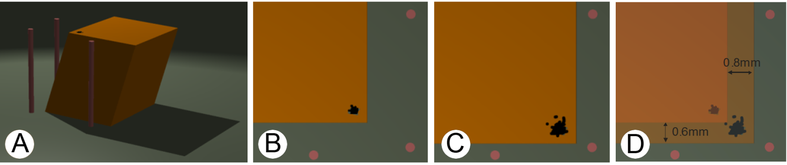
Figure 16. Deskewing example.* A, block prior to grinding with fiduciary edges not at 90 degrees to direction of grinding. B. Serial grinding image #10. C. Serial grinding image #70. D. Movement between B and C.
The vertical cylinders represent fixed points of reference. They will not appear in normal photographs of the fossil as they are too far away (normal images will be zoomed in on this corner for maximum resolution). However, suppose that the images B and C were captured at slices 10 and 70 of the grinding run (at some lower magnification). By overlaying these images (and knowing the scale of the image) we can measure how much the edges have moved over these 60 slices – in this case 0.8mm to the right and 0.6mm downwards. This example is a little artificial, but these sorts of errors do occur in serial grinding datasets, and do require correction.
Deskew values are entered into the mm/Slice Down and mm/Slice Left boxes on the Settings tab of the Output panel. In this example 0.01333 (0.8mm / 60 slices) should be entered for mm/Slice down, and -0.01 (0.6mm / 60 slice) for mm/Slice left - note the use of a negative value for left drift as the edge is actually moving right not left.