3. Basic Concepts
This section contains key introductory information on using SPIERSedit, and is arranged in sequence to guide a new user through the process of constructing and viewing a simple viewable model. More detailed information on the different facilities SPIERSedit provides is provided in later sections.
3.1. How SPIERSedit Stores Data
The data a user supplies to SPIERSedit is an image ‘stack’; a sequence of registered images of consistent resolution. These images are referred to as source images. SPIERSedit does not alter source images, which are retained in their original form as a reference; instead it creates a corresponding stack of working images which it manipulates and uses as the basis for 3D reconstructions. Working images are always grayscale, and may be lower resolution than the source images (see downsampling below). Each dataset has a single SPIERSedit settings file (with a ‘.spe’ extension), which is stored in the same folder as the source images. Working images, together with other files corresponding to each source image, are stored in a subfolder with the same filename as the dataset’s ‘.spe’ file. For example a dataset with a settings file called fossil.spe will have store working images in a folder called fossil. Note that SPIERSedit requires that the working images folder is named in this way – if you rename either folder or settings file the program will not be able to open the dataset.
3.2. Downsampling
Before using SPIERSedit, you will require suitable data using the guidelines provided above. Prior to importing a new dataset you should consider the downsampling required. By default, SPIERSedit creates working images in at the same resolution as source images; for high resolution datasets this may drastically slow SPIERSedit and produce models that are too complex for SPIERSview to visualise. One solution is dataset downsampling, where resolution is divided by an integer factor. For instance, 1000x800 pixel source images might be downsampled by a factor of 4 to produce 250x200 pixel images for reconstruction purposes. Downsampling can also be useful to reduce high-frequency noise. It does of course reduce the detail level in the final model, but in some cases the extra resolution contains little real information, and many CT datasets can safely be downsampled by a factor of 2. Dataset downsampling is defined as a downsample factor within each image (XY downsampling), and a separate factor for averaging between images (Z downsampling). Note that source images are never altered by downsampling or any other SPIERSedit operation. Dataset downsampling has to be defined when creating a new dataset (the default is XY of 1 and Z of 1 - no downsampling); while it is possible to change it later on using the Change downsampling command on the File menu, it is normally preferable to get it right initially! Being able to change this downsampling at a later date allows the majority of preparation work to be done on a downsampled dataset, which can then be upsampled and regenerated. This time-saving technique is outlined later.
3.3. Creating a New Dataset
The first step in making a reconstruction is to import the image stack into SPIERSedit. To do this use the New command on the File menu. Select the source images required for the reconstruction (normally all the images in a particular directory) and click open. In the window which appears (Fig. 1) provide a file name (the more descriptive this is the easier it will be to find in the recently opened files list) and a brief description of the dataset if required. Alter downsample settings if required (see above), and tick the ‘back to front’ box if applicable (see below). Click OK, and after some initial processing a black rectangle will appear. This is the threshold image (see Fig. 2).
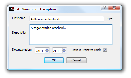
Figure 1. The new dataset window
Is my dataset front-to-back or back-to-front? Tomographic datasets come in two flavours; to understand the difference imagine looking down on top of the specimen, perpendicular to the slice-plane. In a front-to-back dataset the first (i.e. lowest numbered) image is the closest to the viewer, at the top of the specimen; subsequent images move away from the viewer (down the object). Serial-grinding datasets are normally of this type. In a back-to-front dataset the first image is furthest from the viewer, at the bottom of the stack; subsequent images move towards the viewer (up the object). Most CT datasets are of this type. This setting can be changed later on (using the Output panel), but if you get it the wrong way round your model will be mirrored!
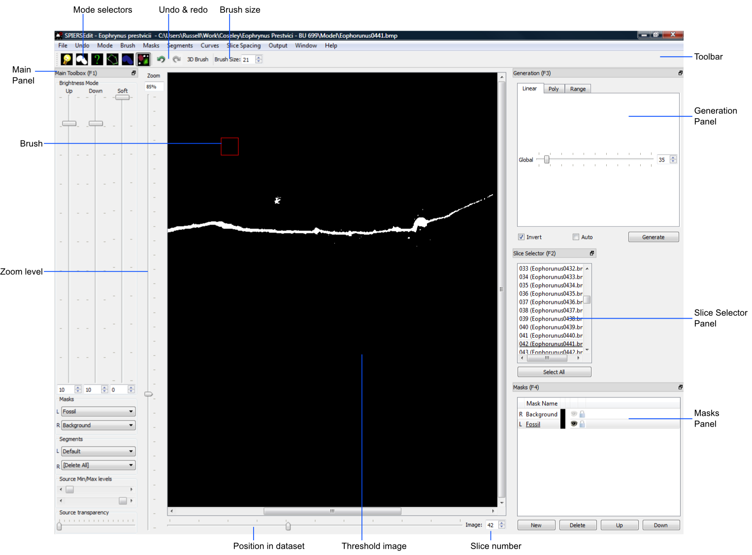
Figure 2. The SPIERSedit default window layout. Note that the GUI and layout shown corresponds to SPIERS 2.X.X. The GUI for 3.X.X employs a dark theme, and has a slightly modified layout, but all instructions in the documentation apply to 3.X.X.
3.5. Threshold image and Linear Generation
The threshold is a binary (black/white) image created from the working image using a simple rule – all working image pixels brighter than mid-grey (index value 128 and above) are treated as on, representing ‘object’ (white), and all pixels darker than this value (127 and below) as off, representing background (black). For palaeontological datasets, ‘object’ normally means fossil, and ‘background’ means matrix (or empty space for isolated specimens). The final three-dimensional model exported to SPIERSview simply consists of all ‘on’ pixels.
Initally all pixels are off, as no proper working images have get been generated; when creating a new dataset SPIERSedit simply generates black ‘dummy’ working images. The first step in handling any new dataset is hence to recalculate working images from source images using appropriate rules; SPIERSedit calls this process Generation, and the appropriate tools are found on the Generation panel.
*To understand how working images, threshold images and simple generation work, the user is strongly advised to run carefully through the following exercise for their first dataset.*
a) Press the Spacebar a few times, noting that this toggles overlay of the source image. Leave the source image on, and alter the zoom with the Zoom level slider so the image fits comfortably onscreen. Note that the keyboard shortcuts for zoom in and zoom out are Q and A respectively.
b) For most datasets the first slice does not contain any specimen; using the Position in dataset slider move to a slice that does; if in doubt move to somewhere near the middle of your dataset.
c) Make sure the Generation panel is visible (see above). On this panel make sure that the tab at the top is set to Linear, leave all the settings at their defaults, and click the Generate button. Nothing will happen initially as you are viewing the source image, but if you press the Spacebar again a few times to flick between source and threshold images you will now see some pixels in white on the threshold image – these are ‘on’ (i.e. SPIERSedit has picked them as ‘object’ using its default rules).
e) With the threshold image visible, try moving the Global slider in the Generation toolbox around to alter the rules used by SPIERSedit to generate the working image; you can either click the Generate button after each change, or tick Auto for changes to be automatically applied as soon as they are made (the latter is normally best, but can be slow for big images and/or slow computers). Note how more or fewer pixels can be turned on by moving the slider. If your images have objects of interest darker than matrix (for instance you want to image voids in a CT dataset), tick the Invert box – try this even if your data are not inverted.
f) In the Mode menu, untick Threshold. This stops SPIERSedit thresholding the image, and shows the underlying working image – alter generation setting again and note how they alter this image. At all times, the threshold image is simply a version of this working image with all pixels darker than mid-grey off, and all pixels lighter than mid-grey on. In normal use you never turn thresholding off, but it is important to understand how the working image underlies the thresholded image. When you are happy, turn thresholding back on.
g) So far we have only generated a working image for one slice. Normal procedure is to determine ‘correct’ settings using a typical slice (see below), then generate working images for the entire dataset. To do this, first ensure the Slice Selector panel is visible, click the Select All button in this panel. Note that all slices are now underlined – All SPIERSedit panels used the convention that underlined = selected. Now click the Generate button in the Generation panel. It may take a few minutes for SPIERSedit to generate working images for the entire dataset. When it has done so, you should be able to move through the dataset and check that all images now have non-blank working images
The Generation panel includes two other tabs, Polynomial and Range; these provide more complex rules for generating working images, and are dealt with under advanced topics. For most datasets, however, linear generation is adequate. Note that for monochrome datasets (e.g. CT), only the Global slider is available, and essentially just controls brightness of the working image. For colour datasets (e.g. from serial grinding) there are also three values for Red, Green and Blue; these are used to weight the contribution of each of the primary colours to the monochrome working image. In most colour datasets there is no need to alter these values from their defaults, but they may occasionally be useful.
Note that while the source image files are never altered, the brightness/contrast with which they are displayed can be modified using the Source Min/Max levels slider in the Main Toolbox panel. The source and threshold images can also be combined using the Source transparency slider in the Main Toolbox panel, allowing the threshold image to be viewed below a semi-transparent source image.
3.6. ‘Correct’ Generation
The goal of Generation is to as near as possible automatically correctly identify which pixels are ‘object’ and which ‘background’; this involves choosing the best settings before generating for the entire dataset. Unless datasets are entirely free from noise there will be no absolutely correct setting, and the goal is to find a setting that is ‘about right’ – i.e. where the edge of the object is being correctly identified as much as possible, and as little background as possible is coming out as white. Toggling between the source and threshold image by using the spacebar is helpful while judging this. Figure 3 shows a colour slice-image from a serial grinding dataset (A), and three attempts at generating a threshold image from it (B-D). Here the fossil is darker than the matrix, so Invert is on. In the first attempt (B), the Global slider is set is too high; although little or none of the matrix is white in the threshold image and much of the fossil is absent. In the second attempt (C) the Global slider is set too low – although most of the fossil is white in the thresholded image, far too much non-fossil material is also coming through. The final attempt (D) is about right – most of the fossil is white and only a little non-fossil material is present.
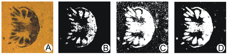
Figure 3. Linear Generation examples. A; source image. B; too dark.(to few white pixels) C; too light (too many white pixels). D; about right.
3.7. Generating Multiple Slices
Clicking Generate (or altering generation settings with Auto ticked) generates new working images for the selected slices. Normally only the currently visible slice is selected, but arbitrary sets of slices can be selected using the Slice Selector panel. For simple datasets (e.g CT) it is only normally necessary to do this once, to all slices, but in some datasets it may be necessary to use different thresholds for different slice ranges. For example, in CT, if the strength of the source varies towards the edge of the detector panel and the first 100 slices and last 100 would need a different global to those in between. For another example, suppose that in a 100-slice serial grinding dataset the lighting conditions had to be changed between slices 50 and 51. In this case, you would generate in two batches – first find good settings for image 1-50, then select those and generate for them. Next, move to image 51 (or anywhere else in the second half), find new settings appropriate for this image, then select images 51-100 and click Generate again.
3.8. Editing Requirements
Almost universally, datasets will need cleaning (here referred to as editing); without any such attention, undesirable scattered ‘on’ pixels and other noise (caused by cracks, artefacts, or other imperfections) will all be rendered into the final model as floating dots, planes, etc. Some relatively faint structures may not be picked out by simple generation rules, and require manual intervention to be identified. Figure 4 shows some typical problems that could be corrected with editing.
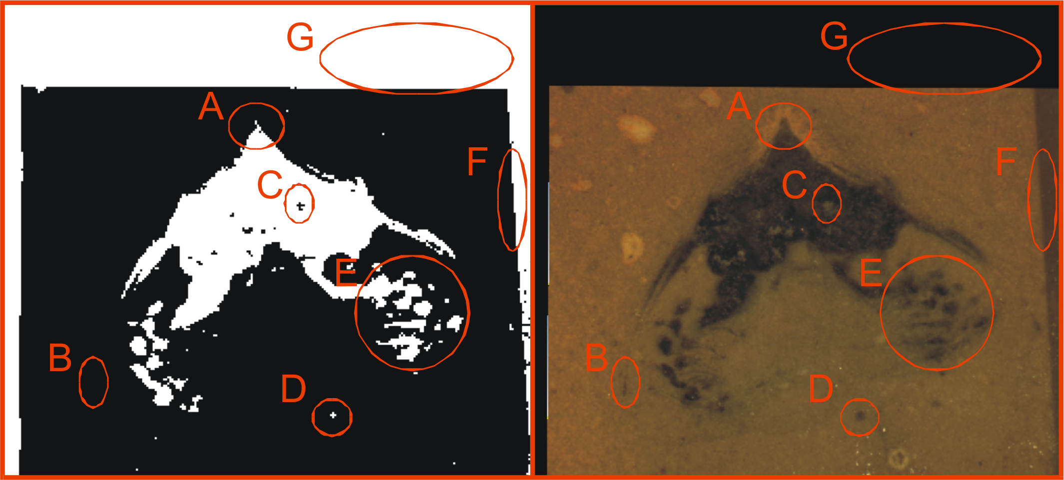
Figure 4. An image requiring editing. Source image is shown on right and thresholded image on left. A; lighter than normal structure not fully picked out. B; Thin structure not picked out at all. C; lighter area of fossil-fill identified as matrix. D; dark blob in the matrix (noise) identified as fossil (this identified by eye as non-fossil by tracing it through several images, and confirming that it does not attach to the rest of the specimen). E; set of structures appearing a ‘fatter’ than they should and merged into each other. F; darker background material misidentified as fossil. G; edge-padding introduced during alignment misidentified as fossil.
Figure 4. An image requiring editing. Source image is shown on right and thresholded image on left. A; lighter than normal structure not fully picked out. B; Thin structure not picked out at all. C; lighter area of fossil-fill identified as matrix. D; dark blob in the matrix (noise) identified as fossil (this identified by eye as non-fossil by tracing it through several images, and confirming that it does not attach to the rest of the specimen). E; set of structures appearing a ‘fatter’ than they should and merged into each other. F; darker background material misidentified as fossil. G; edge-padding introduced during alignment misidentified as fossil.
SPIERSedit does not require editing work to be undertaken; once an initial generation of working images has taken place, any dataset can be output (visualised) – see below. An initial visualisation prior to any editing work is in most cases strongly recommended to better assess the quality of the model possible, and provide a clearer picture of structures which are hard to identify in slice images.
Editing work can be time consuming, especially if done entirely manually with the brush, and involves a degree of interpretation, which could be considered to reduce the objectivity of the data. However carefully edited datasets produce cleaner-looking three-dimensional models, and more importantly can bring out anatomical detail not apparent in ‘raw’ unedited reconstructions, for example thin or impersistent structures. The degree of editing required will depend on the quality of the data, the time available, and the use intended for the resulting model.
Important Note: Noise consisting of small isolated objects (not joined to the main specimen, e.g. error type D is Fig. 4) can be removed automatically using the Island Removal facility of SPIERSview; in many cases this is a much quicker approach than editing the noise out in SPIERSedit.
3.9. Simple Editing
Editing is undertaken by dragging the Brush over the image to alter it. Editing is a per-slice process – what you do only affects the visible slice. It can be performed with or without the source image overlay. The brush appears as a red square or circle (see Fig. 2) superimposed on the image at the current mouse position. Brush options are found in the Brush menu; these include ten preset sizes and a toggle to change between a circular and square brush. Brush size can also be set using the Brush Size spinbox on the menu bar (see Fig. 2). The ‘3D Brush’ setting allows edits to affect multiple slices, and is described later in this document.
The effect of the brush depends on the current mode, indicated (and set) in the mode menu and by the toggle buttons on the toolbar (see Fig. 5). Mode can also be changed using the keyboard shortcuts, which are Ctrl-B (Brightness mode), Ctrl-S (Segment mode), Ctrl-R (Recalc mode), Ctrl-C (Curve mode), Ctrl-L (Lock/selection mode) and Ctrl-M (Mask mode). Brightness, recalc and segment mode are described here (the latter only briefly); a full treatment of segment, Curve, Lock/selection and Mask modes is given later in this document.
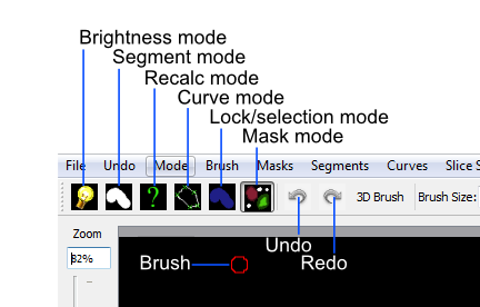
Figure 5. Mode selection toggle buttons.
Brightness mode: allows manual cleaning of data by locally adjusting brightness level of the underlying working image. Brightening (left click / drag) the area under the brush can ‘push’ certain pixels above the threshold level, i.e. turn them ‘on’; this is the best method for ‘bringing out’ structures that are not appearing in the thresholded image as they are a little too dark in the working image (e.g. errors A and B in Fig. 4). Figure 6 shows the effects of brightening – on the left is the brush about to brighten the threshold image shown, and on the right is the threshold image following a single left drag with the brightness brush. Conversely, darkening (right click / drag) will do the opposite, and is the best method for handling regions where too much material is ‘on’ (e.g. error E in Fig. 4).

Figure 6. Effects of brightness brush.
The strength of the brightening and darkening effect from a single brushstroke can be modified using the Up and Down sliders in the Main Toolbox Panel; repeated brush strokes over an area (releasing mouse button between strokes) will strengthen the effect. The brush effect can be ‘feathered’ so it is stronger nearest the brush centre – the Soft slider in the Main Toolbox Panel controls the strength of this feathering effect.
Segment mode: for simple (single-segment) datasets, acts as an ‘on’ and ‘off’ drawing tool; the left mouse button turns pixels on, and the right turns them off. More complex uses of this mode for multi-segment datasets are dealt with below. Left-clicking in segment mode (turning pixels on) could for instance be used to cure error type C in Figure 4, and right-clicking in segment mode (turning pixels off) could be used to cure error types D, F and G. Note that other approaches exist for removing large blocks of material; see Masks section below.
Recalc mode: This re-generates the pixels under the brush using the current generation settings in the Generation Panel, allowing manual application of different generation rules to isolated areas, or a reset of an area to an unedited state.
Undo: the toolbar also incorporates undo controls; Ctrl-Z is the shortcut for undo, and Ctrl-Y is the shortcut for redo. Undo works for editing actions performed using the brush, but not for operations that affect entire slices or groups of slices (e.g. generation).
Tips: editing successfully using the segmentation and especially the brightness brush is an acquired skill, practice will considerably speed a user up! An important trick is to have one hand on the mouse and the other on the keyboard to constantly overlay and remove the source image as a guide (using the spacebar), as well as to switch brush modes and sizes.
3.10. Simple Output (Rendering)
SPIERSedit does not itself handle 3D modelling, but exports its datasets to SPIERSview for viewing in three dimensions. At the simplest level this is done by using the View in SPIERSview command on the Output menu – F12 is the keyboard shortcut. This command initiates an export (which may take an appreciable amount of time), then launches SPIERSview on the exported file. SPIERSview has a separate manual.
In most cases however you will want to review output settings before using the View in SPIERSview command to ensure the model is displayed correctly; these are available in the Settings tab of the Output Panel. The Slices/mm and Pixels/mm boxes are the most important of these settings, specifying the scale and aspect ratio of the output model. Slices/mm is the number of slice images per millimetre in the source dataset; this will be 1/s, where s is the slice-spacing in millimetres. For example if slices are spaced every 40 microns, Slices/mm should be 1 / 0.04 = 25. Pixels/mm is the scale of each (source) slice image, specified as the number of Pixels per millimetre – for instance if the field of view is 3mm and the source image is 300 pixels wide, Pixels/mm should be 100. For CT data and these two values are normally the same, and can be calculated as 1 / v where v is the voxel size (converted to millimetre).
The Sequence front to back tick box is the same ‘front to back’ setting discussed above under Creating a New Dataset.
Other output settings are described later in this manual.
3.11. Saving and Opening Datasets
Saving in SPIERSedit is essentially automatic. Changes made to individual images are made directly to disk. Other information, stored in the ‘.spe’ settings file, is automatically saved when SPIERSedit exits and autosaved by default every five minutes (the Advanced prefs dialog, accesible via the File menu, can be used to change this default). A manual settings save can be triggered at any time using the Save command on the File menu.
SPIERSedit datasets can be re-opened (a) by double-clicking on the SPIERSedit settings file (.spe), (b) by using the Open command on the File menu to open an existing .spe file, or (most conveniently) by using the Open Recent submenu on the File menu. The More… command at the bottom of the Open Recent submenu shows all datasets ever opened by this installation of SPIERSedit.
SPIERSedit does not support multiple datasets – opening a dataset with the Open command will save and close any dataset already open. Multiple copies of SPIERSedit can be opened instead, though be aware that SPIERSedit uses a substantial amount of memory for its file cache (see Advanced Prefs section below), and hence that multiple copies may quickly use up all available system memory.
The Save As command on the File menu creates a second copy of the entire working dataset for backup or other purposes. It does not duplicate the source data files, but creates a new ‘.spe’ file and working dataset folder within the source dataset directory.
The Import SPIERSedit 1.1 command on the File menu is not documented in this manual.
3.12. Advancing Beyond Basic Concepts
The remainder of this manual documents many other features of SPIERSedit. It is recommended that users intending to make extensive use of SPIERSedit read through all these sections, but for those in a hurry the most important sections (in no particular order) are Masks (which allow splitting of a model into colour-coded parts), Segments (which allow for multiple types of material in a model), and Output (which covers how to export and view models with multiple masks and segments).